sometears

library(sometears)
library(ggdag)
library(ggplot2)

Introduction

The sometears package is a collection of functions for estimating directed acyclic graphs (DAGs) from data. The package includes functions for estimating the adjacency matrix of a DAG, thresholding the adjacency matrix, and simulating data from a DAG. The package also includes functions for estimating the structure of a DAG from data, including functions for estimating the adjacency matrix of a DAG, thresholding the adjacency matrix, and simulating data from a simple linear SEM. The two main algorithms that the package implements are the DAGMA algorithm from Bello et al. (2023) and the TOPO algorithm from Deng et al. (2023).

Generate Data

We can generate data from a simple linear SEM using the sim_linear_sem function. This function generates data from a simple linear SEM with a given adjacency matrix $W$ such that value $W_{i,j}$ represents the direct effects from variable $i$ to variable $j$. We assume that the errors are normally distributed with mean 0 and variance $\Sigma = \text{diag}(1)$ such that

$$X = X W + \epsilon \quad \epsilon \sim N(0, \Sigma)$$

$$(I - W)^{-1} X \sim N(0, (I - W)^{-T} \Sigma (I - W)^{-1})$$

set.seed(13)
B <- matrix(
  c(0, 2, 0, 2,
    0, 0, -2, 0,
    0, 0, 0, 2,
    0, 0, 0, 0),
  nrow = 4, ncol = 4, byrow = TRUE)

# Plot the DAG
B_long <- adj_mat_to_long(B)
B_long$name <- B_long$from
ggdag(as_tidy_dagitty(B_long)) +
  theme_void()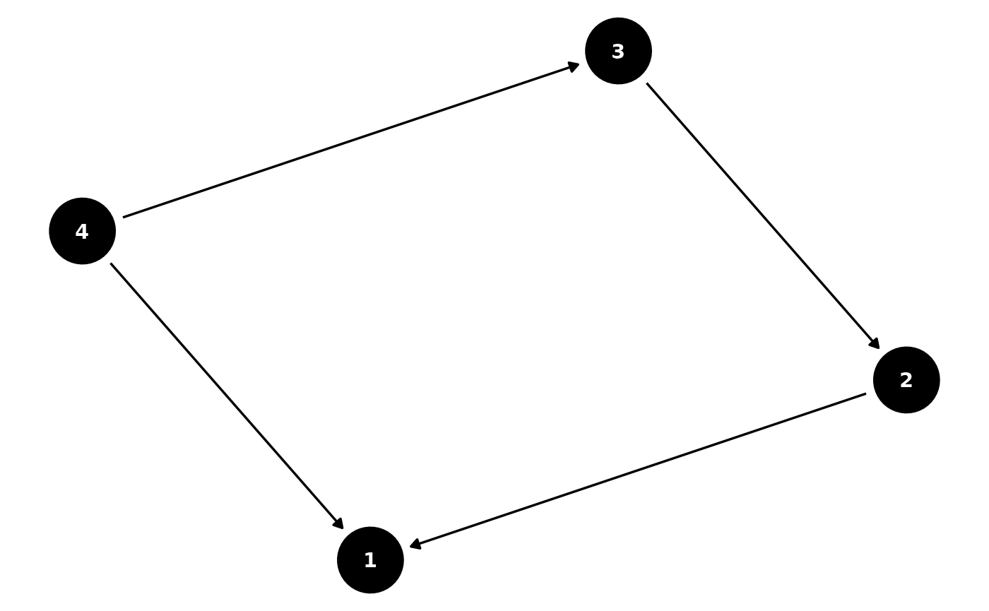

# Simulate from the DAG
d <- ncol(B)
X <- sim_linear_sem(B, n = 500, Sigma = 1 * diag(ncol(B)))

Estimate DAG with DAGMA

DAGMA uses a path-finding algorithm to estimate the adjacency matrix of a DAG. We used the torch package in R to implement the DAGMA algorithm from Bello et al. (2023). Initially we used the ADAM optimizer but found that torch::lbfgs worked better for the algorithm. The algorithm is quite sensitive to the parameters and sometimes can be difficult to converge. This is a limitation of the algorithm and we are working on improving the convergence properties to better align with the python version. Note: This is not evaluated since torch needs to be installed via torch::install_torch

dagma_W <- dagma_fit_linear(
  X,
  trace = T,
  mu = c(1, 0.1, 0.01, 0.001),
  l1_beta = 0.002)
#> Params:  mu: 1, s: 1.1, epoch: 5, l1_beta: 0.002 
#> torch_tensor
#>  0.0993  0.4785 -0.4886  1.1276
#>  0.1768  0.1299 -0.6467 -0.1957
#> -0.1403 -0.1679  0.2113  1.1188
#>  0.0325 -0.0920  0.2253  0.3827
#> [ CPUFloatType{4,4} ][ requires_grad = TRUE ]
#> Params:  mu: 0.1, s: 1.1, epoch: 5, l1_beta: 0.002 
#> torch_tensor
#>  0.0388  1.4284 -0.5675  1.7394
#>  0.0376  0.0502 -1.4493 -0.2000
#> -0.0355 -0.0480  0.0662  1.7507
#> -0.0146 -0.0313  0.0459  0.0643
#> [ CPUFloatType{4,4} ][ requires_grad = TRUE ]
#> Params:  mu: 0.01, s: 1.1, epoch: 5, l1_beta: 0.002 
#> torch_tensor
#>  0.0059  1.9885 -0.1706  1.9246
#>  0.0033  0.0052 -1.9058  0.0156
#> -0.0020 -0.0030  0.0055  1.9915
#> -0.0008 -0.0017  0.0030  0.0053
#> [ CPUFloatType{4,4} ][ requires_grad = TRUE ]
#> Params:  mu: 0.001, s: 1.1, epoch: 5, l1_beta: 0.002 
#> torch_tensor
#>  6.0011e-04  2.0275e+00 -1.4186e-01  1.9360e+00
#>  3.2878e-04  5.1134e-04 -1.9381e+00  3.0202e-02
#> -1.9423e-04 -2.9181e-04  5.4719e-04  2.0087e+00
#> -7.4461e-05 -1.5909e-04  2.9662e-04  5.1541e-04
#> [ CPUFloatType{4,4} ][ requires_grad = TRUE ]

print(round(dagma_W, 2))
#>      [,1] [,2]  [,3] [,4]
#> [1,]    0 2.03 -0.14 1.94
#> [2,]    0 0.00 -1.94 0.03
#> [3,]    0 0.00  0.00 2.01
#> [4,]    0 0.00  0.00 0.00

DAGMA with lbfgs

We also implemented the DAGMA algorithm with the L-BFGS optimizer from the lbfgs package. This adds a better way to do L1 penalty via L-BFGS. We found that the algorithm is still quite sensitive to the parameters and sometimes can be difficult to converge. A very small L1 penalty is needed for the algorithm to converge.

dagma_W <- dagma_fit_linear_optim(
  X,
  trace = T,
  s = 1.1, # logdet penalty
  l1_beta = 0.0001, # Should be small or else it will not converge
  mu = c(1, 0.1, 0.01))
#> Params: mu = 1 , s = 1.1 , l1_beta = 1e-04 
#> Current W:
#>             [,1]        [,2]       [,3]       [,4]
#> [1,]  0.10500959  0.48151367 -0.4275923  1.1438328
#> [2,]  0.18458086  0.12367581 -0.6933266 -0.2055195
#> [3,] -0.14243348 -0.16217341  0.2108205  1.0947227
#> [4,]  0.04183048 -0.09093109  0.2262676  0.3929483
#> Params: mu = 0.1 , s = 1.1 , l1_beta = 1e-04 
#> Current W:
#>             [,1]        [,2]       [,3]        [,4]
#> [1,]  0.03645639  1.44304749 -0.2994723  1.79622853
#> [2,]  0.03359915  0.04996074 -1.6321083 -0.17365325
#> [3,] -0.02704021 -0.04054110  0.0619682  1.76250163
#> [4,] -0.01111610 -0.02655611  0.0427228  0.06513316
#> Params: mu = 0.01 , s = 1.1 , l1_beta = 1e-04 
#> Current W:
#>               [,1]         [,2]         [,3]        [,4]
#> [1,]  0.0049371853  1.910546906  0.000000000 1.904352762
#> [2,]  0.0029219571  0.005447646 -2.028662100 0.000000000
#> [3,] -0.0016009113 -0.003043527  0.005415161 1.964534807
#> [4,] -0.0006340897 -0.001706169  0.003136715 0.005785953

print(round(dagma_W, 2))
#>      [,1] [,2]  [,3] [,4]
#> [1,]    0 1.91  0.00 1.90
#> [2,]    0 0.01 -2.03 0.00
#> [3,]    0 0.00  0.01 1.96
#> [4,]    0 0.00  0.00 0.01

Estimate DAG with TOPO

TOPO swaps pairs in a valid topological order that will decrease the loss function. We find that this algorithm works extremely fast in the linear case and is able to recover the true DAG.

est_B <- fit_topo(X, d:1)
print(round(est_B$W, 3))
#>      [,1]  [,2]   [,3]  [,4]
#> [1,]    0 1.964  0.082 1.945
#> [2,]    0 0.000 -2.088 0.067
#> [3,]    0 0.000  0.000 2.013
#> [4,]    0 0.000  0.000 0.000

Sachs data analysis

data(sachs)
set.seed(1234)

d_sachs <- ncol(sachs)
est_sachs <- fit_topo(as.matrix(sachs), 1:d_sachs, s=1.1)$W

col_names <- colnames(sachs)
result_df <- data.frame(from = character(), to = character(), strength = numeric(), direction = character(), stringsAsFactors = FALSE)
threshold_graph <- 0.5
for (i in 1:nrow(est_sachs)) {
  for (j in 1:ncol(est_sachs)) {
    if ((est_sachs[i, j] > threshold_graph) || (est_sachs[i, j] < -threshold_graph)) {
      new_row <- data.frame(from = col_names[i], to = col_names[j])
      result_df <- rbind(result_df, new_row)
    }
  }
}

if (requireNamespace("bnlearn", quietly = TRUE)) {
  dag <- bnlearn::empty.graph(nodes = colnames(sachs))
  bnlearn::arcs(dag) <- result_df
  bnlearn::graphviz.plot(dag)
} else {
  print(est_sachs)
}
#>              [,1]        [,2]         [,3]        [,4]        [,5]        [,6]
#>  [1,] 0.000000000  0.00000000  0.000000000  0.17194605  0.07877942  0.07385326
#>  [2,] 1.352252378  0.00000000  0.000000000  0.25278685  0.07214880 -0.00900717
#>  [3,] 0.373731358  0.49456100  0.000000000  0.78436901  0.52048313  0.29225973
#>  [4,] 0.000000000  0.00000000  0.000000000  0.00000000  0.00000000  0.00000000
#>  [5,] 0.000000000  0.00000000  0.000000000  0.80603604  0.00000000  0.00000000
#>  [6,] 0.000000000  0.00000000  0.000000000 -0.18228967 -0.08522520  0.00000000
#>  [7,] 0.000000000  0.00000000  0.000000000  0.14364721  0.05793260  0.00000000
#>  [8,] 0.000000000  0.00000000  0.000000000  0.00000000  0.00000000  0.00000000
#>  [9,] 0.006803594 -0.01034267 -0.007080206  0.05773732 -0.02518768  0.07983138
#> [10,] 0.229475400  0.44804562  0.434849430  0.36661795  0.32247086  0.23740054
#> [11,] 0.000000000  0.00000000  0.000000000  0.08633655  0.00000000  0.00000000
#>              [,7]        [,8] [,9]    [,10]      [,11]
#>  [1,]  0.04033524   2.0653899    0 0.000000  0.2553003
#>  [2,] -0.02151390  -0.5569615    0 0.000000 -0.2308707
#>  [3,]  0.13137972   3.1332025    0 0.000000  0.4849756
#>  [4,]  0.00000000   0.1651542    0 0.000000  0.0000000
#>  [5,]  0.00000000   0.2235938    0 0.000000  0.1478282
#>  [6,]  1.40166072 -14.8242956    0 0.000000 -0.2967703
#>  [7,]  0.00000000  12.0324482    0 0.000000  0.2146607
#>  [8,]  0.00000000   0.0000000    0 0.000000  0.0000000
#>  [9,]  0.06345477  -0.2720148    0 1.881136 -1.5427374
#> [10,]  0.12184941   4.6164549    0 0.000000  0.9780254
#> [11,]  0.00000000   0.2590884    0 0.000000  0.0000000